Kernel methods are basically overparameterized linear regression
In this blog post I explain kernel methods and the intuition that they’re “basically just overparameterized linear regression”. First, I will explain what I mean by kernel methods and overparameterized linear regression. I will view them as two methods for solving the following problem:
We are given \(n\) data points \(x_i\) where each data point is a d-dimensional vector. Each data point has a scalar target value \(y_i\). For example, the data points could describe houses by size, location and year of construction and the target value could be the price of the house. Next, we are given a new data point \(z\) (size, location and year of construction of a new house) and want to predict its target value (price of the new house).
Informal description of kernel methods for regression
We may apply a kernel method to this problem as follows:
-
Pick your favorite kernel function k(x,y). Intuitively, this is a function measuring the similarity between x and y, giving higher values to more similar inputs. A popular one is
\[k(x,y) = e^{-\|x-y\|_2^2}.\] -
Build the \(n \times n\) “kernel matrix” by
\[K_{ij} = k(x_i,x_j).\] -
Solve for the coefficient vector \(\alpha\)
\[K \alpha = y.\] -
Calculate similarities to the new data point \(z\) and use this to produce a prediction
\[prediction = \sum_{i=1}^d \alpha_i k(x_i, z).\]
Overparameterized linear regression
Let us now instead apply linear regression to the problem. Since the features \(x_i\) might be related to the target values \(y_i\) in a nonlinear way, it is often useful to preprocess the features before fitting a linear model. For example, if \(x_{i1}\) is the size of house \(i\) and \(x_{i2}\) its year of construction, we might want to add the feature \(x_{i1}\cdot x_{i2}\) to account for nonlinear interactions between \(x_{i1}\) and \(x_{i2}\). Maybe we also want to add something like \(\sin(x_{i2})\) or \(\exp(x_{i1}+x_{i2})\) or the constant value \(1\) (often called intercept). Or we just add all monomials (\(x_{i1}^{p_1}x_{i2}^{p_2}\dots\)) of the input features up to degree \(10\). The possibilities are endless. Let’s assume we processed our old d-dimensional features \(x_i\) into new m-dimensional features \(\tilde{x}_i = \varphi(x_i)\), where \(\varphi\) is our feature transform. Let’s also stack all these new features into a new \(n \times m\) matrix \(\tilde X\). Construct \(\tilde{z} = \varphi(z)\) in the same way.
What if we end up with more features \(m\) than data points \(n\)? This is what we call an overparameterized model. Usually this means we can perfectly fit all the targets \(y_i\). And moreover, we can perfectly fit the targets in many different ways. It makes sense to pick some linear coefficients \(\beta\) such that \(\tilde{X}\beta = y\), i.e we fit the data. And let’s pick the one among those with minimal 2-norm \(\|\beta\|_2\). It turns out that we can calculate this by
\[\beta = \tilde{X}^\top(\tilde{X}\tilde{X}^\top)^{-1}y.\]Then we can make the prediction
\[prediction = \tilde{z} \beta.\]Numerical example
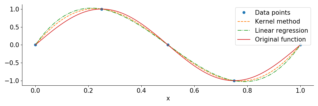
To illustrate the two methods described above, I used them to interpolate the function \(\sin(2\pi x)\) in the interval \(0 \le x \le 1\) from 5 evenly spaced points. In this case the features \(x_i\) are simply the positions of the data points. For the overparamterized linear regression I used the 10 polynomial features \(\left(\frac{x_i}{10}\right)^p\) for \(p = 0,\dots,9\).
Here’s the python code:
import numpy as np
import matplotlib.pyplot as plt

X = np.linspace(0,1,5)   # Training data
y = np.sin(2*np.pi*X)    # Training targets
Z = np.linspace(0,1,100) # Data points to predict

# Kernel method
k = lambda x,y : np.exp(-(x.reshape(-1,1)-y.reshape(1,-1))**2)
K = k(X,X)
alpha = np.linalg.solve(K, y)
kernel_prediction = alpha @ k(X,Z)

# Overparameterized linear regression
features = lambda x : (x.reshape(-1,1) / 10) ** np.arange(10).reshape(1,-1)
X_ = features(X)
beta = X_.transpose() @ np.linalg.solve(X_@X_.transpose(), y)
linear_prediction = features(Z) @ beta

plt.plot(X, y, 'o', label = 'Data points')
plt.plot(Z, kernel_prediction, '--', label = 'Kernel method')
plt.plot(Z, linear_prediction, '-.', label = 'Linear regression')
plt.plot(Z, np.sin(2*np.pi*Z), label = 'Original function')
plt.legend()
plt.show()
Now that I’ve described the two methods, we can get to the point.
Kernel methods are basically overparameterized linear regression
Recall \(\varphi\) as the feature transform taking the old features to the new features in overparameterized linear regression. Now define the kernel function \(k(x,y) = \varphi(x)^\top \varphi(y)\). Then the kernel matrix becomes \(K = \tilde{X}\tilde{X}^\top\) and \(\alpha = K^{-1}y = (\tilde{X}\tilde{X}^\top)^{-1}y\). The final prediction becomes
\[prediction = \tilde{z}\tilde{X}^\top(\tilde{X}\tilde{X}^\top)^{-1}y.\]Does this look familiar? That’s because it is exactly the same prediction that we would get from doing overparameterized linear regression! So if we have a feature transform \(\varphi\), we can construct a corresponding kernel function \(k(x,y) = \varphi(x)^\top \varphi(y)\). What about the converse?
It turns out that under some technical assumptions (look up Mercer’s theorem if you’re interested) on the kernel function \(k(x,y)\), we can find feature transforms \(\varphi\) such that \(k(x,y) \approx \varphi(x)^\top \varphi(y)\) to arbitrary accuracy. And importantly \(\varphi\) can be chosen without knowing the data points \(x_i\) or targets \(y_i\). So the trade-off here is that to get an accurate approximation of \(k(x,y)\) the feature transform \(\varphi\) might output a lot of features.
We may pick some high accuracy \(10^{-100}\), much higher than what we usually compute with, and find some \(\varphi\) such that \(\lvert k(x,y)-\varphi(x)^\top \varphi(y)\rvert < 10^{-100}\) for every relevant x and y. This might require \(10^{10^{10}}\) features, but that’s fine. The point is that overparameterized linear regression on these features is for all practical purposes the same as the kernel method. Note again that the feature transform is independent of \(x_i\) and \(y_i\). Kernel methods hence inherit many properties and limitations of linear regression.
Some applications:
- Linear regression (in view of predictions) only depends on the inner products between data points. For example, duplicating a feature is the same as scaling it up by \(\sqrt 2\), and having features \(x_{i1}\) and \(x_{i2}\) is the same as having features \(\frac{x_{i1}+x_{i2}}{\sqrt 2}\) and \(\frac{x_{i1}-x_{i2}}{\sqrt 2}\).
- In terms of notation, I often find it easier to work with (and think about) a single feature vector for each data point, than considering pair-wise similarities through a kernel function. I feel like it makes it easier to apply linear algebra notation and operations.
- This one is a bit vague: Kernel methods can’t perform “feature learning”, i.e they are stuck with a fixed set of features (given by the kernel function) in a way where they can’t disproportionally focus on the important features. This is in contrast to for example neural networks which we hope will learn good representations of the data useful for transfer learning, ignoring irrelevant features, etc.
If you are interested in this kind of research, I would be happy to talk on Discord, email (johanswi@uio.no), or in the comments below.