Implicit bias by small initialization: A simple classification task where deeper is better
In this blog post I will show an example of implicit bias on a synthetic classification task. I will put code to reproduce the results in spoilers. We will implement everything using pytorch.
Code to import packages
import torch as th
import torch.nn.functional as F
th.manual_seed(0)
import numpy as np
The classification task
Let’s classify \(d = 10\) dimensional input features into \(k = 10\) classes using \(n = 100\) training examples, and generate \(n = 100\) data points for testing.
Code to set constants
d = 10 # Input dimension
k = 10 # Classes
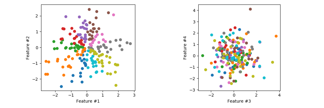
n = 100 # Training examples / testing pointsWe generate independently normally distributed data points in d = 10 dimensions. The classes are determined by the direction of the first 2 dimensions. Note that the other 8 dimensions are only there to confuse the classifier. In the plots below: on the left we see that the classes are separated into 10 pizza slices by angle of the first 2 feature dimensions, on the right we see other dimensions which are useless for classification.
Code to generate data
X = th.randn(n*2, d) # Generate random points
y = ((th.atan2(X[:,0],X[:,1])/np.pi+1)/2*k).long() # Classify points
X_train, y_train = X[:n,:], y[:n] # Train/test split
X_test,  y_test  = X[n:,:], y[n:]
The models
First, let us consider the linear classifier given by a \(d \times k\) matrix \(W\) where we predict the class of the data point \(X\) as the class whose column in \(W\) has the maximum inner product with \(X\), i.e
\[\text{predict}(X) = \text{argmax}_{i \in \{1,\dots,k\}} X \cdot W_i.\]We optimize the model by gradient descent until we have mean cross entropy loss at most 0.01 on the training data. Note that 0.01 cross entropy is quite low, meaning we perfectly fit the training data (100% accuracy), which is only possible since our models are in the overparameterized regime.
Code to train model
def trainModel(parameters, predict, lr):
  loss = 1e100
  while loss > 0.01: # Optimize until mean cross entropy loss is <= 0.01
    loss = F.cross_entropy(predict(X_train), y_train)
    loss.backward()
    with th.no_grad():
      for param in parameters:
        param -= lr * param.grad # Gradient descent
        param.grad[:] = 0
  # Return test accuracy
  return th.sum(th.argmax(predict(X_test), dim=1) == y_test).item()
We can now train the simple linear model.
Code to test simple linear model
W = th.zeros(d,k, requires_grad=True)
parameters = [W]
predict = lambda X : X@W
print("Test accurracy:", trainModel(parameters, predict, lr=10), '%')
We get an accuracy of 53%. The hyperparameters for learning rate (lr) and stopping threshold (0.01) don’t seem to matter much if they are small enough (but making them smaller takes more time to optimize).
Let us now apply the rule of thumb from deep learning that “deeper is better” and add another layer. We parameterize \(W = AB\) for a \(d \times k\) matrix \(A\) and \(k\times k\) matrix \(B\).
\[\text{predict}(X) = \text{argmax}_{i \in \{1,\dots,k\}} X \cdot [AB]_i.\]For the previous parameterization, the optimization problem was convex, but this time it is not. This means initialization matters (in particular, if we initialize \(A = B = 0\) we will have gradient 0 and not get anywhere), let’s therefore initialize by a standard initialization from deep learning called Xavier/Glorot normal initialization. Let us also run 10 times to average out the random initialization.
Code to test 2 layer model
scores = []
for _ in range(10):
  A = th.zeros(d,k, requires_grad=True)
  B = th.zeros(k,k, requires_grad=True)
  th.nn.init.xavier_normal_(A) # Equivalent to A = th.randn(d,k)*(2/(d+k))**.5
  th.nn.init.xavier_normal_(B) # Equivalent to B = th.randn(k,k)*(2/(k+k))**.5
  parameters = [A,B]
  predict = lambda X : X@A@B
  scores.append(trainModel(parameters, predict, lr=1))
print("Test accurracy: %.1f ± %.1f %%"%(np.mean(scores), np.std(scores)/len(scores)**.5))
We get an accuracy of 60.3% with standard deviation 0.6%. The accuracy improved! How can this happen? Classical intuition tells us that parameterizing a matrix as a product of matrices is useless, as we can only represent exactly the same set of classifiers. The key is that we are in the overparameterized regime, where gradient descent has many solutions to choose from. The parameterization changes the implicit bias of the model when it is trained by gradient descent, causing it to choose a different solution.
Let’s go deeper!
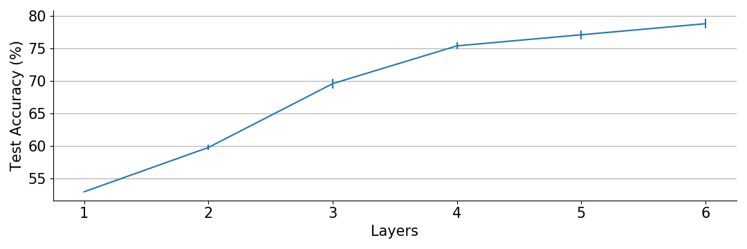
Clearly more layers give better accuracy.
Code to test models of various depths
for L in [1,2,3,4,5,6]:
  scores = []
  for _ in range(10):
    layers = []
    for l in range(L):
      layers.append( th.zeros(d if l==0 else k, k, requires_grad=True) )
      th.nn.init.xavier_normal_(layers[l])

    def predict(X):
      product = X
      for layer in layers: product @= layer
      return product

    if L == 1: lr = 10
    elif L == 2: lr = 1
    else: lr = 3e-2
    scores.append(trainModel(layers, predict, lr))
  print("Test accurracy: %.1f ± %.1f %%"%(np.mean(scores), np.std(scores)/len(scores)**.5))
The explanation
To understand why depth improves generalization accuracy, we need to note that our classification problem has “low rank” in a certain sense. Consider the optimal classifier matrix \(W\) with respect to
\[\text{predict}(X) = \text{argmax}_{i \in \{1,\dots,k\}} X \cdot W_i.\]The i’th column (so the direction of class i-1 in the 0-indexed code) of this matrix is given by \(W_i = \left(\sin\left(\frac{\pi(2i-1-k)}{k}\right), \cos\left(\frac{\pi(2i-1-k)}{k}\right), 0, \dots, 0\right)^\top\). Note that since only the first two rows of \(W\) are non-zero, we have \(\text{rank}(W) = 2\). Intuitively, there are much fewer matrices with rank 2 than general matrices, so if we can somehow implicitly bias our model towards low rank matrices (or preferably rank 2 matrices), we will likely get better classification accuracy.
To demonstrate, let’s explicitly force \(W\) to be rank 2 by factoring it into a \(d \times 2\) matrix \(A\) and a \(2 \times k\) matrix \(B\) so \(W = AB\), and then repeat our experiment.
Code to test rank 2 model
scores = []
for _ in range(10):
  A = th.zeros(d,2, requires_grad=True)
  B = th.zeros(2,k, requires_grad=True)
  th.nn.init.xavier_normal_(A)
  th.nn.init.xavier_normal_(B)
  parameters = [A,B]
  predict = lambda X : X@A@B
  scores.append(trainModel(parameters, predict, lr=1))
print("Test accurracy: %.1f ± %.1f %%"%(np.mean(scores), np.std(scores)/len(scores)**.5))
85% accuracy! That’s the best we’ve seen. Ok, but our other deep factorizations didn’t force the matrix to be low rank, so how did they exploit the low rank property?
That is most easily seen if we scale down the outputs of a three layer factorization \(W = \frac{1}{10^4}ABC\).
Code for near-zero initialized three layer factorization
scores = []
for _ in range(10):
  A = th.zeros(d,k, requires_grad=True)
  B = th.zeros(k,k, requires_grad=True)
  C = th.zeros(k,k, requires_grad=True)
  th.nn.init.xavier_normal_(A)
  th.nn.init.xavier_normal_(B)
  th.nn.init.xavier_normal_(C)
  parameters = [A,B,C]
  predict = lambda X : X@A@B@C / 1e4
  scores.append(trainModel(parameters, predict, lr=100))
print("Test accurracy: %.1f ± %.1f %%"%(np.mean(scores), np.std(scores)/len(scores)**.5))
We get an accuracy of ca 84%. Plotting the singular values of the product matrix \(\frac{1}{10^4}ABC\) during training, we see what is going on.
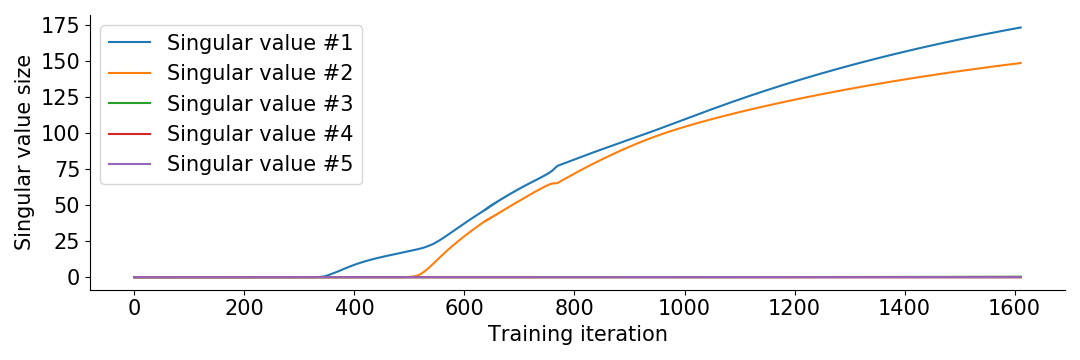
We see that the singular values show up one by one. When only the first singular value is non-negligible, we are effectively searching through rank 1 matrices. After a while it introduces the next singular value to search rank 2 matrices. Then the optimization terminates because it fits the training data. The remaining singular values are left around the initialization magnitude \(\frac{1}{10^4}\).
In contrast to scaling down the outputs, if we switch \(\frac{1}{10^4}\) to \(10^3\) so \(W = 10^3 ABC\) (and adapt the learning rate to lr = 0.001), we get accuracy 57.5% with standard deviation 1%. So we are back down to accuracies around the one layer case, since we removed most of the implicit bias.
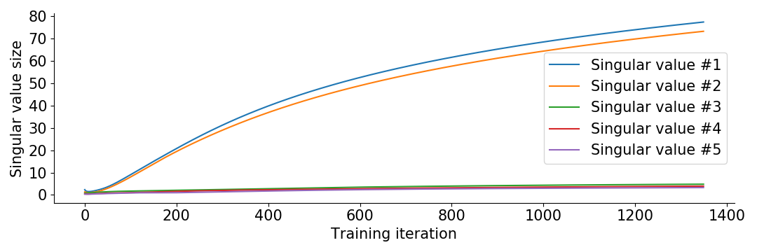
Now you might wonder how we got any benefit from depth in our original setup, where we seemingly didn’t have small initialization. The clue is that it is really the relative size of initialization to final size which determines whether we are in the “small initialization regime”. Since our overfitting of the cross entropy loss results in the final matrix \(W = ABC\) having singular values around size 100, the initialization of size around 1 becomes small in comparison. You can see this in the following plot of the evolution of singular values for the original 3 layer model.
The implicit bias demonstrated in this blog has many names given by different researchers, such as near-zero / small initialization regime, following “saddle-to-saddle” dynamics, anti-NTK regime and rich regime / rich limit. The experiment itself was motivated by Arora’s paper on Implicit Regularization in Deep Matrix Factorization. In that paper, they describe the differential equations for the singular values and what causes them to show up one by one to give the low rank implicit bias. Simply put, increasing the depth causes the effect to strengthen. The experiment in this paper is an adaptation of their experiment from matrix completion to classification.
If you are interested in this kind of research, I would be happy to talk on Discord, email (johanswi@uio.no), or in the comments below.