Implicit bias in single epoch SGD
Large transformer models are typically trained using only a single epoch, i.e the model only sees each data point once. Theoretically, this training regime circumvents problems related to overfitting and generalization by converting them to a question of how fast we can converge given noisy gradients.
My recent experiments indicate that the implicit bias by small initialization is important in this regime, also in quite realistic settings. This makes me hopeful that the single epoch training SGD regime is a good setting to study several important phenomena observed in deep learning. In this blog I will showcase single epoch training on the following matrix sensing task.
Matrix sensing task
Our task is to estimate a \(d\times d\) ground truth matrix \(T\). The effect we are studying in this blog is more apparent at larger scales, so we pick the fairly large dimension \(d \in \{256,1024\}\). We generate \(T\) as a random matrix of rank \(r \in \{2,5\}\).
The \(i\)th training example consists of a \(d\)-dimensional input vector \(a_i\), a \(d\)-dimensional vector \(b_i\) of output weights, and a scalar target value \(y_i = a_i^\top T b_i\).
We let \(a_i\) and \(b_i\) be random Gaussians \(a_i, b_i \sim \mathcal{N}(0,I)\). To make \(T\) of rank \(r\), we generate it as the product of two random Gaussian matrices of sizes \(d\times r\) and \(r \times d\).
Simple setting
In this section, I will describe one of the simplest settings I know where the implicit bias is apparent. Then, in later sections I will show more realistic settings.
Our simple model will be a 2 layer linear network (as in this previous post). The parameters are two \(d\times d\) matrices \(W_1\) and \(W_2\). The model outputs \(\mathrm{predict}(a_i,b_i) = a_i^\top W_1 W_2 b_i\). We use the squared sample loss \(L_i = \frac{1}{2}(y_i-\mathrm{predict}(a_i,b_i))^2\). The parameters are initialized using Xavier normal initialization (random Gaussians with scale \(\frac{1}{\sqrt d}\)).
We train the model by SGD with constant learning rate \(\eta\), for a single epoch. This means we loop through the samples one by one, for each taking a step of length \(\eta\) along the negative gradient of \(L_i\). Note that we need a large enough learning rate \(\eta\) to be able to converge after only one epoch. A too small learning rate will keep the weights too close to the initialization, making learning impossible. However, a too large learning rate will make the model diverge.
We will be exploiting implicit bias by small initialization. Actually, instead of scaling down the initialization, we will scale up the target values, which is equivalent (for homogeneous models like ours). Therefore, we add a parameter \(\gamma\) which sets the scale of the ground truth matrix \(\gamma T\).
We pick \(d = 256\), \(r = 2\), \(\eta = 2\times 10^{-8}\) and \(\gamma = 100\).
Code for simple setting
import torch as th
import matplotlib.pyplot as plt
th.manual_seed(0)

d = 256      # Input and output dimension
r = 2        # Rank of ground truth matrix
lr = 2e-8    # Learning rate
yscale = 100 # Scale factor for ground truth

T = th.randn(d,r)@th.randn(r,d) * yscale

W1 = th.randn(d,d, requires_grad=True)
W2 = th.randn(d,d, requires_grad=True)
th.nn.init.xavier_normal_(W1)
th.nn.init.xavier_normal_(W2)

log = []
for i in range(d*d//2):
  a, b = th.randn(d), th.randn(d)
  loss = 0.5*(a@T@b-a@W1@W2@b)**2
  loss.backward()
  with th.no_grad():
    for param in [W1,W2]:
      param -= lr * param.grad # Gradient descent
      param.grad[:] = 0
  if i%100 == 0:
    error = (W1@W2-T).norm()/T.norm() # Relative error
    log.append((i,error))

plt.plot(*zip(*log))
plt.show()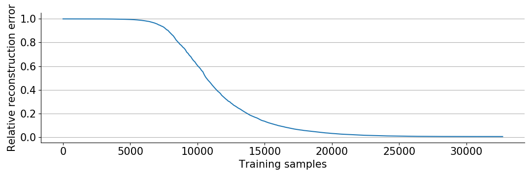
Without exploiting the rank constraint, and using only \(\frac{1}{2}d^2\) samples, we would expect a relative reconstruction error (Frobenius norm of \(W_1W_2-T\) over Frobenius norm of \(T\)) of around \(0.5\). However, we only ran the optimization long enough to see \(\frac{1}{2}d^2\) samples, and as seen in the plot above we already converged and reconstructed the correct matrix!
More realistic setting
What interests me about the setting above, i.e single epoch SGD with low rank linear ground truth, is that we can observe the same phenomena in much more realistic settings. We can add more layers, non-linearities, even normalization layers, and we still see the same phenomena!
The first “realistic” setup is what I call “the CNN setup”. Typical CNNs (like ResNet and PyramidNet) use ReLU(-like) activation functions, batch normalization, and are optimized by SGD with momentum. Our model consists of 10 layers with ReLU non-linearities and Batch Normalization, optimized by SGD with momentum.
The second “realistic” setup, I call “the transformer setup”. Transformers typically use ReLU-like activations, layer normalization, and are optimized by the Adam optimizer. We stack 10 layers with ReLU activations and layer normalization, and optimize by Adam with default parameters.
We also scale up the experiment a bit to \(d = 1024\), \(r = 5\) and use mini-batches of size \(256\) to speed up the computations.
Code for more realistic setting
import matplotlib.pyplot as plt
from tqdm import tqdm # Optional loading bar
import torch as th
nn = th.nn
F = nn.functional
th.manual_seed(0)

device = 'cuda'
#device = 'cpu'

d = 1024      # Input and output dimension
r = 5         # Rank of ground truth matrix
B = 256       # Batch size
L = 10        # Number of layers
yscale = 4e-2 # Scale factor for ground truth

truth = (th.randn(d,r)@th.randn(r,d)).to(device) * yscale

cnn = nn.Sequential(*[x for i in range(L) for x in [nn.Linear(d,d,bias=False), nn.BatchNorm1d(d), nn.ReLU()]][:-2]).to(device)
sgd = th.optim.SGD(cnn.parameters(), lr=2.5e-8, momentum=0.9)

transformer = nn.Sequential(*[x for i in range(L) for x in [nn.Linear(d,d,bias=False), nn.ReLU(), nn.LayerNorm(d)]][:-2]).to(device)
adam = th.optim.Adam(transformer.parameters(), lr=6e-4)

for net,opt,label in [(cnn,sgd,'CNN'), (transformer,adam,'Transformer')]:
  log = []
  for bi in tqdm(range(0, d**2//2, B)):
    a = th.randn(B, d, device=device)
    b = th.randn(B, d, device=device)
    y    = th.einsum('bi,bi->b', a@truth, b)
    pred = th.einsum('bi,bi->b', net(a), b)
    loss = th.sum((y-pred)**2)

    log.append((bi, (loss/th.sum(y**2)).item() ))

    opt.zero_grad()
    loss.backward()
    opt.step()

  plt.plot(*zip(*log), label=label)
plt.legend()
plt.show()
Interesting phenomena
While performing experiments like the ones above, I recognized numerous phenomena seen elsewhere in deep learning. This makes me hopeful that this simple setting is a good place to study and understand phenomena which are otherwise hard to specify and analyze.
Small initialization / large targets
Implicit bias by small initialization seems crucial to the experiments. If the initialization is too large compared to the ground truth (so \(\gamma\) too small), all the networks seem unable to train quickly and generalize. Interestingly, while the simple settings require very large \(\gamma\), the more realistic settings (more layers, normalization layers) work best with smaller values of \(\gamma\). When doing classification instead of regression, the standard classification losses (say cross entropy with label smoothing) have a slightly larger target scale by default. That could mean we don’t need any explicit target scaling. We saw this effect in a previous blog post.
Only works well for large instances
Deep learning is very data hungry, with simpler methods beating it when data is scarce. The single epoch training regime might shed some light on why that is, as it also only works for large instances.
Learning rate warm-up
In practical deep learning, “learning rate warm-up” is an important trick where we gradually increase the learning rate at the start of training. By using this trick, I was able to use larger learning rates later without diverging. For example, we can add opt.param_groups[0]['lr'] = 1e-7*min(1,0.1+bi/(d**2/4)) before opt.step() in the CNN setting.
Normalization layers
Normalization layers seem to help train deeper networks. However, it is not well understood why. Maybe analyzing the effect of normalization layers in this simple setting can give some insights.
Theory
The theory of online optimization is well suited to describe single epoch SGD. As a brief introduction to online optimization, I will give a simple proof of how single epoch SGD optimizes convex functions. The proof is mostly taken from “Convex Optimization: Algorithms and Complexity” by Sébastien Bubeck.
We want to optimize the differentiable (or we could work with subgradients), convex function \(\tilde f \colon \mathbb{R}^d \to \mathbb{R}\). To apply SGD, we sample from some family of differentiable functions \(f \colon \mathbb{R}^d \to \mathbb{R}\) satisfying \(\mathbb{E}\|\nabla f\|_2^2 \le B^2\) and \(\mathbb{E}\nabla f = \nabla \tilde f\). Next, we assume there exists some minimizer \(x^* \in \mathbb{R}\) of \(\tilde f\), and we have some initial guess \(x^1\). The SGD update rule is
\[x^{k+1} = x^k-\eta\nabla f^k(x^k),\]where \(f^k\) is randomly sampled.
By convexity \(\tilde f(x^k) - \tilde f(x^*) \le \nabla \tilde f(x^k)^\top(x^k-x^*)\). So
\[\begin{align*} \mathbb{E}\min_{k \in \{1,\dots,K\}} \tilde f(x^k) - \tilde f(x^*) \le \frac{1}{K} \mathbb{E}\sum_{k=1}^K \tilde f(x^k) - \tilde f(x^*)\\ \le \frac{1}{K} \mathbb{E}\sum_{k=1}^K \nabla \tilde f(x^k)^\top (x^k-x^*) = \frac{1}{K} \mathbb{E}\sum_{k=1}^K \nabla f^k(x^k)^\top (x^k-x^*) \end{align*}\]Using \(x^{k+1}-x^k = -\eta\nabla f^k(x^k)\) and \(2u^\top v = \|u\|_2^2+\|v\|_v^2-\|u-v\|_2^2\), we calculate
\[\begin{align*} \nabla f^k(x^k)^\top (x^k-x^*) &= \frac{1}{\eta}(x^k-x^{k+1})^\top (x^k-x^*)\\ &= \frac{1}{2\eta}(\|x^k-x^{k+1}\|_2^2+\|x^k-x^*\|_2^2-\|x^*-x^{k+1}\|_2^2)\\ &= \frac{1}{2\eta}(\|x^k-x^*\|_2^2-\|x^{k+1}-x^*\|_2^2)+\frac{\eta}{2}\|\nabla f(x^k)\|_2^2 \end{align*}\]Inserting into the previous expression, we get a telescoping sum. We pick \(\eta = \frac{\|x^1-x^*\|_2}{B\sqrt K}\) to minimize the final bound. Hence
\[\begin{align*} &\frac{1}{K} \mathbb{E}\sum_{k=1}^K \nabla f^k(x^k)^\top (x^k-x^*)\\ = &\frac{1}{2K\eta} \mathbb{E}\left(\|x^1-x^*\|_2^2-\|x^{K+1}-x^*\|_2^2\right) + \frac{\eta}{2K}\mathbb{E}\sum_{k=1}^K \|\nabla f(x^k)\|_2^2\\ \le &\frac{1}{2K\eta} \|x^1-x^*\|_2^2 + \frac{\eta B^2}{2} = \frac{\|x^1-x^*\|_2B}{\sqrt K}. \end{align*}\]In summary, \(\mathbb{E}\min_{k \in \{1,\dots,K\}} \tilde f(x^k) - \tilde f(x^*) \le \frac{\|x^1-x^*\|_2B}{\sqrt K}\). This shows that in expectation, we successfully optimize the function with rate \(\frac{1}{\sqrt K}\).
If you are interested in this kind of research, I would be happy to talk on Discord, email (johanswi@uio.no), or in the comments below.