94% on CIFAR-10 in 94 lines and 94 seconds
The following code scores 94.02% test accuracy (mean of 40 runs) in 94 lines and less than 94 seconds training time (loading / validation / etc. not included). My tests were performed on NVIDIA A10 GPUs, with pytorch version 1.12.1+cu116 and torchvision version 0.13.1+cu116.
Code
import torch, torchvision, sys, time, numpy
from torch import nn
import torch.nn.functional as F

device = torch.device("cuda")
dtype = torch.float16

EPOCHS = 24
BATCH_SIZE = 512
MOMENTUM = 0.9
WEIGHT_DECAY = 5e-4*BATCH_SIZE
lr_knots = [0, EPOCHS/5, EPOCHS]
lr_vals  = [0.1/BATCH_SIZE, 0.6/BATCH_SIZE, 0]
W,H = 32,32
CUTSIZE = 8
CROPSIZE = 4

class CNN(nn.Module):
  def __init__(self):
    super().__init__()

    dims = [3,64,128,128,128,256,512,512,512]
    seq = []
    for i in range(len(dims)-1):
      c_in,c_out = dims[i],dims[i+1]
      seq.append( nn.Conv2d(in_channels=c_in, out_channels=c_out, kernel_size=(3,3), stride=(1,1), padding=(1,1), bias=False) )
      if c_out == c_in * 2:
        seq.append( nn.MaxPool2d(2) )
      seq.append( nn.BatchNorm2d(c_out) )
      seq.append( nn.CELU(alpha=0.075) )
    self.seq = nn.Sequential(*seq, nn.MaxPool2d(4), nn.Flatten(), nn.Linear(dims[-1], 10, bias=False))

  def forward(self, x, y):
    x = self.seq(x) / 8
    return F.cross_entropy(x, y, reduction='none', label_smoothing=0.2), (x.argmax(dim=1) == y)*100

def loadCIFAR10(device):
  train = torchvision.datasets.CIFAR10(root="./data", train=True, download=True)
  test  = torchvision.datasets.CIFAR10(root="./data", train=False, download=True)
  ret = [torch.tensor(i, device=device) for i in (train.data, train.targets, test.data, test.targets)]
  std, mean = torch.std_mean(ret[0].float(),dim=(0,1,2),unbiased=True,keepdim=True)
  for i in [0,2]: ret[i] = ((ret[i]-mean)/std).to(dtype).permute(0,3,1,2)
  return ret

def getBatches(X,y, istrain):
  if istrain:
    perm = torch.randperm(len(X), device=device)
    X,y = X[perm],y[perm]

    Crop = ([(y0,x0) for x0 in range(CROPSIZE+1) for y0 in range(CROPSIZE+1)],
        lambda img, y0, x0 : nn.ReflectionPad2d(CROPSIZE)(img)[..., y0:y0+H, x0:x0+W])
    FlipLR = ([(True,),(False,)],
        lambda img, choice : torch.flip(img,[-1]) if choice else img)
    def cutout(img,y0,x0):
      img[..., y0:y0+CUTSIZE, x0:x0+CUTSIZE] = 0
      return img
    Cutout = ([(y0,x0) for x0 in range(W+1-CUTSIZE) for y0 in range(H+1-CUTSIZE)], cutout)

    for options, transform in (Crop, FlipLR, Cutout):
      optioni = torch.randint(len(options),(len(X),), device=device)
      for i in range(len(options)):
        X[optioni==i] = transform(X[optioni==i], *options[i])

  return ((X[i:i+BATCH_SIZE], y[i:i+BATCH_SIZE]) for i in range(0,len(X) - istrain*(len(X)%BATCH_SIZE),BATCH_SIZE))


X_train, y_train, X_test, y_test = loadCIFAR10(device)

model = CNN().to(dtype).to(device)
opt = torch.optim.SGD(model.parameters(), lr=0, momentum=MOMENTUM, weight_decay=WEIGHT_DECAY, nesterov=True)

training_time = stepi = 0
for epoch in range(EPOCHS):
  start_time = time.perf_counter()
  train_losses, train_accs = [], []
  model.train()
  for X,y in getBatches(X_train,y_train, True):
    stepi += 1
    opt.param_groups[0]['lr'] = numpy.interp([stepi/(len(X_train)//BATCH_SIZE)], lr_knots, lr_vals)[0]

    loss,acc = model(X,y)
    model.zero_grad()
    loss.sum().backward()
    opt.step()
    train_losses.append(loss.detach())
    train_accs.append(acc.detach())
  training_time += time.perf_counter()-start_time

  model.eval()
  with torch.no_grad():
    test_accs = [model(X,y)[1].detach() for X,y in getBatches(X_test,y_test, False)]

  summary = lambda l : torch.mean(torch.cat(l).float())
  print(f'epoch % 2d  train loss %.3f  train acc %.2f  test acc %.2f  training time %.2f'%(epoch+1, summary(train_losses), summary(train_accs), summary(test_accs), training_time))
Why 94%? Because that’s reportedly human level accuracy on CIFAR-10. Additionally, it made for a reasonable balance between accuracy, code complexity and training time.
The code and idea is based on the final code from the fantastic blog series How to Train Your ResNet from myrtle.ai. The blog series worked on optimizing the training time to reach 94% on CIFAR-10, and was able to get it down to 26 seconds!
The code from myrtle.ai ended up being more than 500 lines long and containing a large number of clever tricks and optimizations.
Motivation
My main interest is in studying why deep learning works so well, specifically the implicit biases of deep learning. Ideally, I would like to study and do experiments on realistic and representative models and tasks. However, it’s not actually clear what is realistic and representative of deep learning. The best criterion seems to be “it works much better than all approaches not based on deep learning”.
However, the best performing deep learning models are also the largest (taking days to train on hardware I don’t have access to) and full of tricks which make them impossible to analyze mathematically and hard to even reproduce. I am therefore interested in finding the simplest cases where deep learning works significantly better than alternative approaches. Image classification on CIFAR-10 is among the best I’ve found for these criteria.
myrtle.ai’s model was a good starting point, as it reduced training time from hours to seconds, when compared to most alternatives. However, many of the tricks they used would complicates analysis while only providing a small gain in performance. I removed many of the less significant optimizations in favor of simplicity. Things like “frozen batch norm scales” and “exponential moving averages” were removed.
You might think that reducing training time to seconds is overkill, since taking some minutes to train a model sounds fine. However, it is very useful to have some wiggle room in training time. As an example, the final accuracy varies from run to run because of randomness in the training procedure (data augmentation, initialization), so myrtle.ai typically did 50 runs just to reduce this variance.
The important tricks
While trying to simplify the code, I found the following tricks to be critical for performance.
Batch normalization
Basically, everything diverges if you remove normalization layers in modern deep learning models. Without normalization layers, things like initialization size, learning rate and layer scaling become fragile hyperparameters. In general, it seems that even when all these (new) hyperparameters are tuned well, it’s too hard to compete with batch norm. The myrtle.ai blog came to a similar conclusion.
Data augmentation
Without data augmentations, accuracies drop to around 90%, which is not significantly better non-deep learning approaches.
I believe the current best non-deep learning methods for CIFAR-10 are convolutional kernel methods, which are typically based on linearizing neural network architectures. These can reach around 90% accuracy on CIFAR-10 (89%, 90%), but struggle for large training sets. They need an \(N \times N\) Gram matrix, where \(N\) is the number of training samples. This means they cannot use data augmentation to the same degree as modern deep learning.
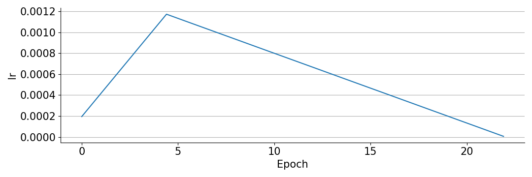
Learning rate schedule / warm-up
I used this learning rate schedule:
Interesting observations
Residual connections were not necessary
I expected residual connections to be crucial for the network architecture. However, they were not necessary, so I removed them.
Output scale is important
The code from myrtle.ai scales down the output of their model by a factor 8. This is very interesting to me, since this is a trick to increase the effect of what I call “implicit bias by small initialization”. I used the trick myself in previous blogs like 1 and 2.
If you are interested in this kind of research, I would be happy to talk on Discord, email (johanswi@uio.no), or in the comments below.